Recently, I have been working on a problem of contour detection in images. Naturally, I started with the Canny edge detection algorithm to get an edge map, hoping to fit the desired curve equations to subsets of the detected edge pixels. My problem was, however, that an edge map doesn’t provide a natural way to “walk along” its edges. The reason is that the familiar 4-connected and 8-connected neighborhoods don’t work well when dealing with edges.
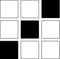
The 4-connected approach would make diagonally lying pixels disconnected, for example:

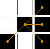
On the other hand, the 8-connected approach would result in spurious additional connections like this:

How can we define a connectivity pattern that gives more satisfactory results when dealing with edges? I found interesting ideas in Peter Kovesi’s MATLAB codes that suggested a possible answer.
The first step is to define the concept of a crossing. Pick an edge pixel and consider its eight surrounding pixels whose values we label \(P_0, P_1, …, P_7\).
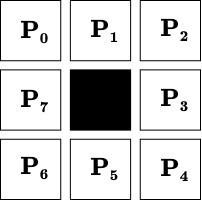
We say that a crossing occurs whenever \(P_i \ne P_{i+1}\) (including the case \(P_0 \ne P_7\) ). Here are a few examples of edge pixel configurations where the crossings are marked with dashed lines:
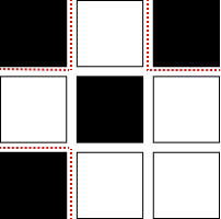
\(N=6\) crossings
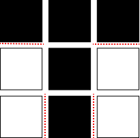
\(N=4\) crossings
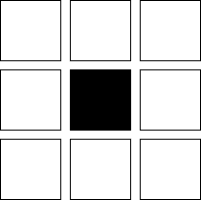
\(N=0\) crossings
We can quickly convince ourselves that the number of crossings, \(N\), must always be even. Each pixel can, therefore, be characterized by the number \(m=\frac{N}{2} \), which, for reasons that will shortly become apparent, we’ll call the degree of the pixel. Let’s agree on a taxonomy, part of which I borrowed from Peter Kovesi:
- Pixels with \(m = 0\) will be called isolated
- Pixels with \(m = 1\) will be called ends
- Pixels with \(m = 2\) will be called links
- Pixels with \(m = 3\) will be called 3-junctions
- Pixels with \(m = 4\) will be called 4-junctions
Let’s draw the connectivity pattern we want for each case above. They should look like this:
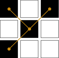


In the cases above, we can convince ourselves that the number \(m\) (half the number of crossings) indeed equals the degree of the central pixel in the connectivity graph. There are cases where we don’t know how the connectivity pattern should look, but it seems that the number-of-crossings taxonomy doesn’t make sense. For example:

\(m=1 \rightarrow \) “end”?
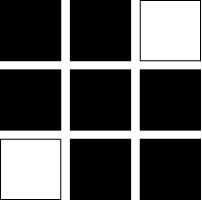
\(m=2 \rightarrow \) “link”?

\(m=0 \rightarrow \) “isolated”???
We need to define what a “wedge” is to exclude such cases. Using the pixel notation from above, if any of the pixel sets \( \{P_7, P_0, P_1\}\), \(\{P_1, P_2, P_3\}\), \(\{P_3, P_4, P_5\}\), or \(\{P_5, P_6, P_7\}\) consists entirely of edge pixels, we’ll call such a set a wedge. For example, in case (d), the wedges are: \( \{P_7, P_0, P_1\}\) and \(\{P_5, P_6, P_7\}\):
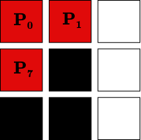

From now on, we will assume that our edge map doesn’t contain any edge pixels with wedges around them. We can do this because, in practice, the Canny edge detector returns very few such edge pixels, and we scan the resulting edge map line-by-line and greedily remove any edge pixel with wedges around it.
A “wedge-free” edge map allows us to formally define the desired connectivity type, which we’ll call nearest-neighbor connectivity. First, let’s separate the diagonal neighbors: \(P_0, P_2, P_4, P_6\) from the boundary neighbors: \(P_1, P_3, P_5, P_7\). Then, under nearest-neighbor connectivity, an edge pixel is connected to a diagonal neighbor only if it has no corresponding boundary neighbors. Otherwise, it is to be connected to its boundary neighbors.
For example, it is to be connected to \(P_0\) if the latter is an edge pixel and neither \(P_1\) or \(P_7\) are edge pixels themselves. The connectivity patterns for cases (a) and (b) above demonstrate this idea. Here is another example:

When using this type of connectivity, half the number of crossings, \(m\), perfectly agrees with the pixel degree in the connectivity graph.
In the upcoming posts, I’ll discuss efficient implementations of the above algorithm and possible applications for contour detection.
